Shipping NibNet: Bringing Food Recognition On-Device
PyTorch
CORE ML
CV
iOS
The Cost of a Cloud-Backed Food Camera
A cloud-based food camera incurs two costs on every scan: inference spend and user wait time. The user takes a photo of their lunch, the app returns a dish name and a macro breakdown, and the entry lands in the day's calorie log. Behind that surface, the work runs in a data center: a multipart POST to a Vercel-hosted backend, a GPT-class vision model parsing the image, a structured response coming back over the wire. The described architecture is simple, making it easy to ship, but the resulting latency and inference costs are less attractive.
Measured on a real device (TestFlight v1.3.x running on an iPhone 15 Pro across 40 representative meal images), every cloud call burns roughly 3,750 tokens at a backend rate of 2M tokens per dollar, which works out to ~$0.002 of LLM spend per scan. The round trip averages 5.2 seconds end to end, with the p50 (median latency) sitting around 4.9s and the p95 (tail latency) above 6s. The unit cost looks small, but the unit latency can be noticeable. An app processing an average of 50,000 daily scans burns through about $2,810 a month in cloud inference, and accumulates somewhere between 220,000 and 300,000 seconds of user-facing latency per day.
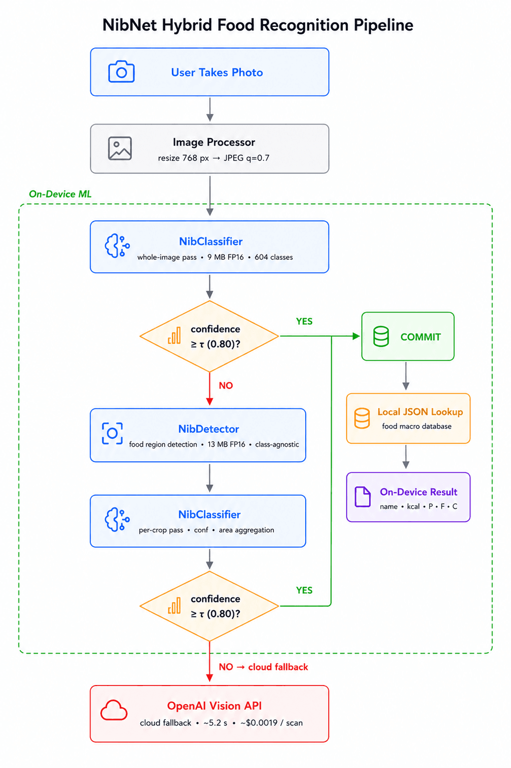
To improve both the token cost and latency performance we developed NibNet, a 23 MB hybrid on-device model shipping inside Nibby, an iOS calorie tracker. Inside it, a fine-tuned MobileNetV4-Conv-Small classifier handles the full image first; when confidence falls below threshold, it routes to NibDet, a custom anchor-free food detector built from scratch after no open-source candidate cleared the licensing and size requirements simultaneously. Both components run on the Apple Neural Engine. This configuration handles 42.6% of scans on-device at 0.883 precision and a 5.0% confidently-wrong rate, in 22 ms at p50 (220× faster than the cloud round-trip) at zero token cost; the remaining 57.4% fall back to the existing cloud LLM route. End to end, the hybrid cuts average latency by ~42% and per-scan cost by ~45%. The chain of decisions that produced this result is described in detail in the following sections.
The Constraints That Shaped the Approach
One: Model size and compute speed. The total food recognition payload had to stay under 50 MB to avoid materially affecting the app's download weight. Size and inference latency are coupled on mobile: a model that clears the accuracy bar but adds hundreds of milliseconds to p50 has traded one UX problem for another. The Apple Neural Engine accelerates a known op set; architectures that don't convert cleanly land on CPU instead. Stock timm model MobileNetV4-Conv-Small converts cleanly and runs on ANE; architectures that don't were considered, then disqualified.
Two: Confidently-wrong is unrecoverable. Hallucinating "fettuccine alfredo" when the user consumed "cauliflower rice" can undermine trust in the app, while falling back to cloud inference with a slower response is more acceptable. The existing cloud LLM picks up whatever the on-device path declines to answer. So the safety bar for the on-device part is set very conservatively to wrong-confident ≤ 5%, prioritizing prediction reliability over maximum recall.
Three: ~600 food classes is a sweet spot, not an arbitrary cap. More food classes in a mobile classification model means more confusion between visually similar dishes: a MobileNetV4-class backbone can't reliably separate paneer_tikka from chicken_tikka on visual cues alone. The practical ceiling under a wrong-confident safety constraint lands in the low hundreds. Every predicted label also has to map to a macro table row, so the class set and the product surface are coupled. The final label space settled at 604 canonical classes: large enough to cover common foods, small enough to remain visually distinguishable.
The following development pipeline has emerged from those constraints :
Detector Selection: Built NibDet from scratch under Apache 2.0 to clear size (≤ 25 MB FP32) and license requirements.
Classifier Fine-Tuning: Fine-tuned MobileNetV4-Conv-Small, MobileNetV3-Large, and MobileCLIP2-S0 on a locked 604-class taxonomy.
Bench Evaluation: Scored eight pipeline variants using a Pareto sweep to find the optimal confidence threshold τ.
CoreML Conversion: Validated strict FP16 agreement gates against the PyTorch reference before any model ships.
Real-Device Validation: Measured latency, cost, and routing behavior on a TestFlight build.
Choosing the Right Metric
The third step listed above includes a Pareto sweep, which requires carefully selected evaluation metrics. Before the detector or the classifier, the evaluation framework has to be defined, because it determines what "winning" means for every pipeline that follows. Top-1 accuracy would have given the wrong answer here.
A model that says "I don't know" 80% of the time and is right 95% of the time it does speak is safer in production than a model that's 70% accurate on every input. The first model commits less and is right when it commits; the second commits constantly and is wrong about a third of the time. In a calorie-tracking UX where a more sophisticated cloud LLM is already available as a backstop, the first model is wiser: it stays quiet when uncertain and lets the cloud handle the hard ones. Top-1 accuracy can't see that difference. It scores both models on the same axis and rewards the chatty one.
Therefore three metrics replaced top-1 accuracy, with the fourth one (precision) only provided as a reference, each a direct echo of a decision the production routing logic actually makes. Let GT be the ground-truth class set for an image (cardinality ≥ 1) and P be the set the on-device path commits to (after applying threshold τ and the conservative pruning rule below). The formula for each metric is summarized under the formula column of the table below.
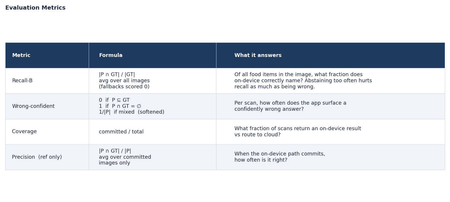
Recall-B gives partial credit on multi-item plates: one correct label on a two-item plate scores 0.5, two correct labels score 1.0. Fallbacks contribute 0 to the average, so a model that abstains on 80% of images cannot exceed Recall-B = 0.20 regardless of how accurate it is on the 20% it commits.
Coverage measures the fraction of scans committed on-device and is only meaningful when Wrong-confident remains under the 5% cap.
The optimization framing follows from the constraints. Maximize Recall-B subject to pooled Wrong-confident ≤ 0.05. Every candidate gets the lowest τ in the allowed range that keeps wrong-confident under the cap. That's the most permissive operating point that still respects the trust floor; raising τ further only sacrifices Recall-B without buying more safety. The 5% wrong-confident cap is the user-trust contract: a model that exceeds it isn't just slightly worse, it's disqualified.
Worked example. A three-class plate (rice, chicken, broccoli). The model commits to {rice, chicken, fettuccine}. |P| = 3, |GT| = 3, |P ∩ GT| = 2. Precision = 2/3, Recall-B = 2/3, Wrong-confident = 1/3 under the softened rule, where a hallucinated label inside an otherwise-correct list is partially redeemed because the user also sees two correct items. The same image scored under binary-wrong would have counted 1.0 on the wrong axis, which is exactly the over-penalization the softened rule is designed to fix.
1. The Detector Selection
The first step of building a composite food recognition model is selecting a deployable detector. Three pipeline modes were on the table (classifier-only, detector-always-on, and hybrid), and none of the detector-dependent ones could be evaluated without a shippable candidate in the pool. For this application, that meant clearing three criteria simultaneously: Apache 2.0 license, ≤ 25 MB FP32, and ≥ 0.49 mAP@.50. Four detectors went through the evaluation:
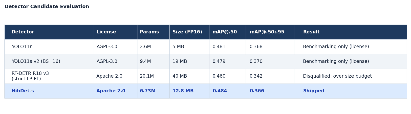
NibDet is a YOLO-inspired clean-room implementation under Apache 2.0 so it can ship inside a closed-source iOS binary. The detector localizes; the classifier names the dish. At 12.8 MB FP16, it is about a third of RT-DETR's size at higher mAP.
Both YOLO entries were retained as benchmarking baselines for the composite pipeline evaluation, where the license constraint doesn't apply.
On AGPL-3.0 and closed-source mobile. AGPL treats network-mediated use of derived software as triggering the same source-availability requirement as distribution. An AGPL detector embedded in an iOS binary would require the entire app's source to be made available to every user who runs it.
RT-DETR was the strongest Apache-2.0 candidate at the time of evaluation. It cleared the accuracy gate (0.460 mAP@.50) but not the size ceiling: at 40 MB FP16, it ran more than 1.5× over budget.
NibDet was trained on a 50k/3.8k/11.4k train/val/test split derived from Open Images V7 and shipped as a 12.8 MB FP16 checkpoint.
2. The Classifier Journey: Eight Pipelines
Before getting to the pipelines, we needed to determine the classifier head dimension. The classifier ships a 604-class output layer, where each class is a canonical food name with a row in the macro lookup table. Those 604 classes were built by unifying Food-101 and several publicly available international food image datasets; across roughly 750 source labels, deduplication and canonicalization collapsed to 604 classes with each mapping cleanly to calories, protein, fat, and carbs. The unified corpus totaled 500,269 images, split as 85/10/5 into train, val, and test.
Following the taxonomy curation with 604 final classes, eight production-eligible pipelines went through the bench, where the fine-tuned classifier models were reduced down to two main options:
Two classifier-only candidates:
mnv3_6hc(MobileNetV3-Large),mobileclip_6hc(MobileCLIP2-S0 image tower).Six detector + classifier composites: mixing RT-DETR-R18 and YOLO11s with the MobileCLIP, MNV3, and NibNet heads.
Hybrid mode for each composite model: run the classifier on the whole image first, and only invoke the detector + per-crop classification when the classifier's confidence falls below threshold.
nibnet_6hc_v2 came out of three rounds of warm-start training. Each round preserved the food-adapted backbone, reinitialized the classification head when the taxonomy changed, and then fine-tuned end-to-end on the updated label space.
The final 20-epoch fine-tune lifted validation top-1 from 0.5469 at epoch 0 to 0.7139 at epoch 16, with top-5 reaching 0.9188. These metrics served primarily as training-health indicators, confirming that the warm-start strategy, augmentation pipeline, and taxonomy corrections were working as intended. They were not used for model selection. The production problem was not maximizing classification accuracy in isolation, but deciding when an on-device prediction should be trusted enough to avoid a cloud fallback. EMA tracking (β=0.9999) captured the gains before late-epoch noise pulled the raw weights backward.
Training used AdamW with cosine schedule, label smoothing, MixUp, class-balanced sampling, and AMP over 20 epochs. Warm-starts converge fast when the backbone is already food-adapted; longer schedules added EMA drift without lifting the validation curve.
3. Benchmark Evaluation with a Stratified Test Set
Aggregate metrics can be misleading and this is where more granularity helps clarify the picture. A pooled 0.913 precision is consistent with "near-perfect on easy images, much weaker on hard ones," and the difference matters a lot in production. So the bench stratified its 594 held-out test images (drawn from the 604-class taxonomy) into four buckets, each one a different failure mode:
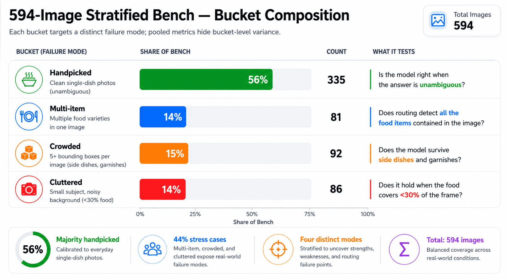
For nibnet_6hc_v2 hybrid mode at τ = 0.80, per-bucket Recall-B lands at 0.499 handpicked, 0.099 multi-item, 0.166 crowded, 0.256 cluttered. The handpicked bucket carries the highest commit rate (~52%) at near-zero wrong-confident (2.1%); the multi-item and crowded buckets sit in the 10-17% Recall-B range. Wrong-confident climbs with clutter: 2.1% on handpicked, 8.7% on crowded, 11.0% on cluttered.
The pooled wrong-confident rate meets the 5% target, but bucket-level performance varies substantially. Cluttered images reach 11% wrong-confident, highlighting a potential traffic-mix risk if production data differs from the benchmark distribution.
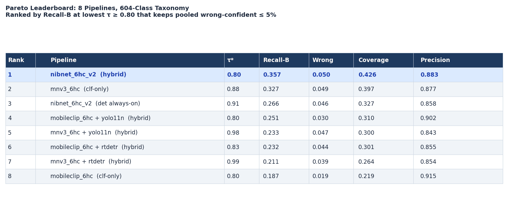
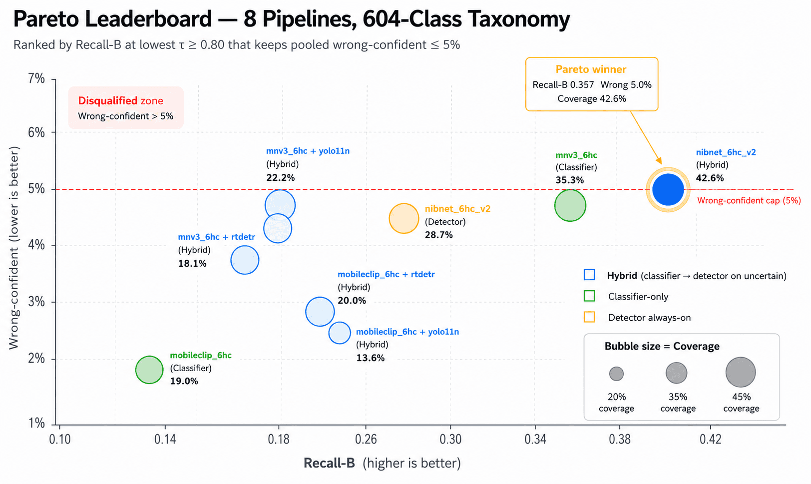
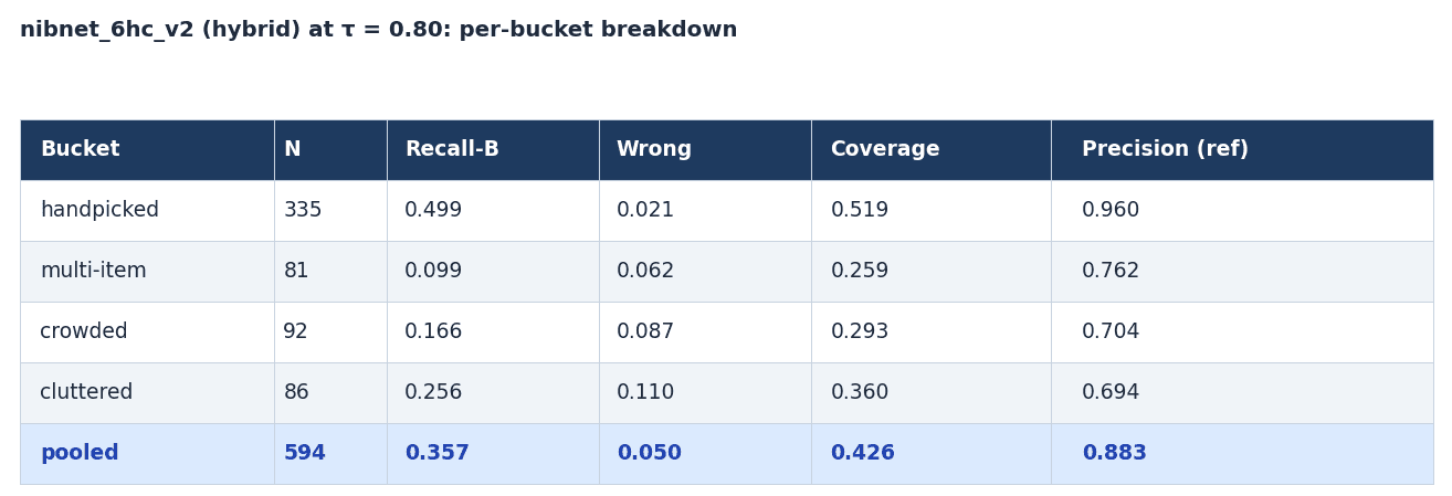
The hybrid's value over running the detector on every image (det always-on, rank 3) is +9.1 pp pooled Recall-B and +2.5 pp Precision. The gain is largest on handpicked images (+14.7 pp Recall-B): the whole-image classifier handles clean single-dish photos without ever invoking the detector, committing faster and more accurately. Of the 42.6% of scans that go on-device, 30.8% are committed by the classifier alone and 11.8% are committed via the detector path. The detector is reserved for the uncertain cases, not applied to everything.
On the shipping threshold. The Pareto sweep was run with a minimum τ floor of 0.80 to absorb FP16 CoreML conversion drift and real-world traffic-mix uncertainty. The nibnet_6hc_v2 hybrid pipeline wins at τ* = 0.80 (Recall-B = 0.357). The threshold is remote-config tunable and will be revisited once production telemetry confirms the safety margin holds.
4. CoreML Conversion, the Hybrid Router, and iOS Deployment
A model that trains well and benches well still has to land inside a production app without any of its measured properties degrading in the process. That transition from a PyTorch checkpoint to a CoreML mlpackage running inside an iOS binary is where subtle things tend to go wrong quietly. Three details in this layer required more attention than their apparent size suggested.
The PyTorch ↔ CoreML agreement gate. Before any mlpackage lands in Copy Bundle Resources, a validation step compares CoreML outputs against the PyTorch reference on a 200-image fixture set. The bar: top-1 agreement ≥ 99% and max absolute delta ≤ 1e-3 in FP16. The 1e-3 threshold is calibrated: normalization bugs show at 1e-1 to 1e-2, pure FP16 drift at 1e-5, so 1e-3 is where systematic problems become visible without noise catching every PR. coremltools can fold normalization into the graph in ways the calling code doesn't expect; the gate catches that at conversion time. Conversion that fails is a release blocker, not a soft warning.
Preprocessing recipe is the number-one silent-failure risk. The training-time transform is resize 224 × 1.15 (= 258) → center-crop 224 → ImageNet mean/std normalize. Any deviation quietly drops top-1 agreement 10-20%. The mitigation is testClassifierAgreesWithBenchJSONL, a Swift test that asserts byte-for-byte label equality against PyTorch reference predictions on a small fixture suite. Without it, preprocessing drift is invisible: the model returns a prediction, just systematically the wrong one, and bench numbers stop matching production within the first day of use.
Remote-config flags ship with the binary. Three flags drive the router. onDeviceRecognitionEnabled is the master kill switch. onDeviceDetectionEnabled ships false and can be flipped for a cohort A/B test without a new build. onDeviceClassifierThreshold is τ, defaulting to 0.80 and tunable once telemetry confirms the safety margin holds. A debug-only forceRouteToCloud flag exists for incident response; if the on-device path misbehaves, the entire path can be disabled in under five minutes and every active user picks up the change on their next foreground.
5. What Shipped, and What's Next
The on-device results are provided in the table below. These measurements are taken from a TestFlight v1.3.x build running on an iPhone 15 Pro, averaged across a 40-image evaluation set drawn from the production scan distribution.
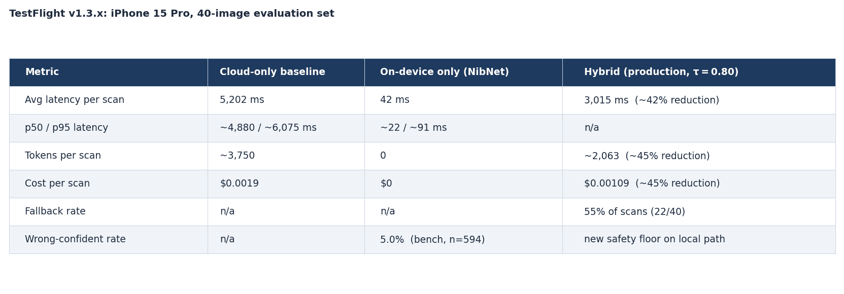
The TestFlight set (n=40) is too small to be authoritative on wrong-confident; so the bench figure of 5.0% across 594 images is the production target.
The side-by-side screen capture video at the top of this page illustrates the latency difference between the on-device ML vs Cloud API operation modes. For 50,000 daily scans (~1.5M/month), cloud-only inference costs about $2,810/month; the hybrid path drops that to about $1,550/month, a ~$1,260/month delta that scales linearly with usage.
The 42 ms figure is steady-state; cold start runs ~422 ms because CoreML lazy-loads the mlpackage. The 55% fallback rate reflects a conservative τ = 0.80 chosen for safety margin; production telemetry will determine whether it can be lowered.
Lessons from the build
Design the metric before the model. Top-1 accuracy would have selected the wrong architecture in this application. The three-metric framing (Recall-B, wrong-confident, coverage) plus a Pareto threshold sweep disqualified candidates that looked good on raw accuracy but exceeded the wrong-confident cap in production conditions.
A small model can create a large product impact. NibNet's 23 MB footprint enabled a 45% reduction in cloud inference cost and a 42% reduction in average latency. In this deployment setting, efficiency mattered more than raw model capacity.
Stratify the bench by failure mode. A pooled metric hides orders of magnitude of variance. The four-bucket bench surfaced a wrong-rate climb from near-zero on clean single-dish photos to 10% on cluttered scenes before any user saw it. That asymmetry is what production calibration has to handle.
The detector module worked best as a specialist, not a default. Running the object detector on every image ranked third in the benchmark. The winning pipeline used a whole-image classifier for easy cases and invoked the detector only when confidence fell below threshold. This hybrid strategy improved Recall-B by 9.1 points and Precision by 2.5 points relative to running the detector on every image.
What's next
The two open questions are the ANE-vs-CPU story on older A-series silicon (A15 / A14) and whether the bench's bucket mix holds against real traffic. A multi-device latency run across A15 and A14 can answer the first question; and a two-to-four-week production telemetry read will settle the second. If wrong-confident rates stay under the 5% cap, τ can be lowered incrementally (0.80 → 0.75 → 0.70) to increase on-device coverage.
Published May 2026
Alper Erten, Applied ML engineer and co-founder of Hus Collective, the company behind Nibby, a calorie tracker for iPhone.
Go back home